A new type of electrical air breakdown, called runaway breakdown or runaway discharge, was discussed recently by Gurevich et al. [1992] and applied to the preliminary breakdown phase of a lightning discharge. This phase occurs in the cloud vicinity and marks the initiation of the discharge [Uman, 1987]. The important property of the runaway breakdown is that it requires a threshold field by an order of magnitude smaller than the conventional breakdown discharge under the same pressure conditions. However, its initiation depends on the presence of seed electrons with energy in excess of tens keV in the high electric field region. Such energetic electrons are often present in the atmosphere as secondaries generated by cosmic rays [Daniel and Stephens, 1974].
The possibility for influence of cosmic ray secondaries on the lightning discharges was first discussed in a speculative manner by Wilson [1924]. Recently McCarthy and Parks [1992] attributed X-rays observed by aircrafts in association with the effect of thundercloud electric field on runaway electrons. Gurevich et al. [1992] presented the first consistent analytic and numerical model of the runaway discharge and later on Roussel-Dupre et al. [1994] presented its detailed quantitative application to the X-ray observations.
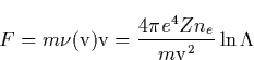
The physics of the runaway discharge is based on the concept of electron
runaway acceleration in the presence of a laminar electric field [Dreicer, 1960; Gurevich, 1960; Lebedev, 1965]. The
runaway phenomenon is a consequence of the long range, small angle
scattering among charged particles undergoing Coulomb interactions. The
scattering cross section decreases with velocity as ![]() [Jackson 1975]. As a result for a given electric field value
a threshold energy can be found beyond which the dynamic friction, as shown
in Fig (5.1), cannot balance the acceleration force due to the
electric field resulting in continuous electron acceleration.
[Jackson 1975]. As a result for a given electric field value
a threshold energy can be found beyond which the dynamic friction, as shown
in Fig (5.1), cannot balance the acceleration force due to the
electric field resulting in continuous electron acceleration.
![\begin{figure}
\center
\includegraphics [width=4in,height=4in]{images/run_1.eps}\end{figure}](img267.gif) |
Here we review the basic physics of the electron runaway in unmagnetized
plasmas, starting with the electron acceleration in a fully ionized plasma.
The cold electrons having mean directed velocity v less than the electron
thermal speed ![]() undergo the dynamical friction force
undergo the dynamical friction force
![]()
 |
(11) |
A similar situation occurs in a weakly ionized plasma. But unlike the fully
ionized plasma, the collision frequency of the low velocities electrons in
the weakly ionized gas is determined by the cross-section of the
electron-neutral collision, rather than by the thermal electrons. However,
for electrons with energies in excess of the ionization potential (![]() ) the interactions with the nuclei and atomic electrons obey
the Coulomb law, hence the dynamical friction force decreases with the
electron energy, [Bethe and Ashkin, 1953] as given by Eq. (5.1 ). In this case the value of the critical electric field is given by
Gurevich, [1960]
) the interactions with the nuclei and atomic electrons obey
the Coulomb law, hence the dynamical friction force decreases with the
electron energy, [Bethe and Ashkin, 1953] as given by Eq. (5.1 ). In this case the value of the critical electric field is given by
Gurevich, [1960]
We emphasize that the amplitude of the electric field leading to the
electron runaway is limited, since only for nonrelativistic electrons the
dynamical friction force drops when the electron energy increases [Bethe and Ashkin, 1953]. For the electrons having energy greater than ![]() keV the dynamical friction force due to collisions with
the neutral gas is given by [Bethe and Ashkin, 1953]
keV the dynamical friction force due to collisions with
the neutral gas is given by [Bethe and Ashkin, 1953]
 |
(12) |
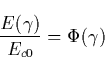
The detailed discussion of the electron runaway in the air caused by the electric fields due to thunderstorm is presented by McCarthy and Parks [1992]. A new step in the theory of runaway electrons was made by Gurevich et al. [1992], who discussed the possibility of producing an avalanche of runaway electrons. The basic idea is that the fast electrons ionize the gas molecules producing a number of free electrons. Some of secondary electrons have energy higher than the critical energy of runaway. Those electrons are accelerated by the electric field and in turn are able to generate a new generation of fast electrons. This avalanche-like reproduction of fast electrons is accompanied by the exponential increase of the number of thermal secondary electrons, i.e. the electrical breakdown of gas occurs. Such kind of the runaway breakdown is often called runaway discharge. It has the following main properties:
These properties allow us to consider the runaway discharge as the possible mechanism which initializes the lightning discharge during thunderstorms.
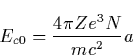
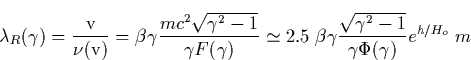
To help with future calculations, we note that the value of the critical
electric field as a function of altitude is given by ![]() V/m, where
V/m, where ![]() km
is the atmospheric scale height.
km
is the atmospheric scale height.
As the friction force becomes smaller with height, the magnetic field must
be included in the analysis. This is especially true for the equatorial
regions where the laminar electric field due to lightning is predominantly
perpendicular to the magnetic field [Papadopoulos et al., 1996].
Note that in the case of E![]() B, a geometry expected in the equatorial
region, the electrons will be accelerated only when E>B, if we neglect the
dynamical friction. Suppose we first neglect the dynamical friction and
quantify what is the E field required to produce infinite acceleration for a
given E, B configuration where
B, a geometry expected in the equatorial
region, the electrons will be accelerated only when E>B, if we neglect the
dynamical friction. Suppose we first neglect the dynamical friction and
quantify what is the E field required to produce infinite acceleration for a
given E, B configuration where ![]() is the angle
between the electric and geomagnetic fields.
is the angle
between the electric and geomagnetic fields.
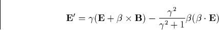
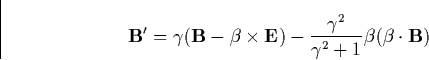
We follow Papadopoulos et al., [1996] and study the runaway acceleration of
a test electron in crossed static electric and magnetic fields by
transforming the equations of motion to a reference frame moving with the
velocity ![]() relative to the ionospheric frame in which the
transformed fields E
relative to the ionospheric frame in which the
transformed fields E![]() , B
, B![]() are
parallel. In this frame the electrons can be treated as unmagnetized.
Following Jackson [1975] the electric and magnetic field in a
moving frame are
are
parallel. In this frame the electrons can be treated as unmagnetized.
Following Jackson [1975] the electric and magnetic field in a
moving frame are
 |
(13) |
 |
(14) |
![]()
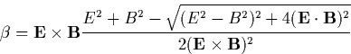
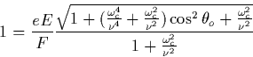
![\begin{displaymath}
E^{\prime 2}=\frac 12[E^2-B^2+\sqrt{(E^2-B^2)^2+4(\mathbf{E\cdot B})}] \end{displaymath}](img316.gif)
![\begin{displaymath}
B^{\prime 2}=\frac 12[B^2-E^2+\sqrt{(E^2-B^2)^2+4(\mathbf{E\cdot B})}] \end{displaymath}](img317.gif)
As a result there is not acceleration in the case of crossed electric and
magnetic field with B>E. Therefore, the characteristic electric field in
SI units is ![]() where B is the local magnetic
induction. Since at the equator the magnetic field is B=0.25 G, the
required field accelerate an electron corresponds to
where B is the local magnetic
induction. Since at the equator the magnetic field is B=0.25 G, the
required field accelerate an electron corresponds to ![]() .This threshold applies to the condition that
.This threshold applies to the condition that ![]() which is
the situation for electrons above a thunderstorm close to the equator.
which is
the situation for electrons above a thunderstorm close to the equator.
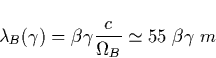
This threshold field is also independent of height at long as the gyroradius
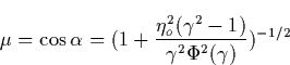
is smaller than the mean free path of runaways which occurs at altitudes as
low as 25 km for sensible electric fields [Longmire, 1978; Papadopoulos et al., 1994]. The above results can be extended to any angle
between the electric and magnetic fields. In the parallel frame, the ![]() field still needs to beat the coulomb friction force, i.e.
field still needs to beat the coulomb friction force, i.e. ![]() . Figure (5.2) shows the condition in
the
. Figure (5.2) shows the condition in
the ![]() plane where
plane where ![]() . Note the
constraint at
. Note the
constraint at ![]() .
.
This is a qualitative analysis, that constraints the field to a threshold
value ![]() which seems to be a characteristic threshold
in the presence of the Earth's magnetic field. Of course the Coulomb
friction term is not covariant, hence, its frame transformation is far from
trivial. The detailed quantitative approach will be presented in the
following sections.
which seems to be a characteristic threshold
in the presence of the Earth's magnetic field. Of course the Coulomb
friction term is not covariant, hence, its frame transformation is far from
trivial. The detailed quantitative approach will be presented in the
following sections.
The Boltzmann equation for the high energy (![]() keV) electron
distribution function where the interactions are primary Coulomb in nature
can be written as [Roussel-Dupre et al., 1994]
keV) electron
distribution function where the interactions are primary Coulomb in nature
can be written as [Roussel-Dupre et al., 1994]
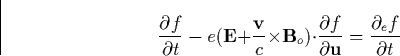 |
(15) |
![\begin{displaymath}
\frac{\partial _ef}{\partial t}=\frac 1{\mathrm{u}^2}\frac{\...
...ial {\partial \mu }[(1-\mu ^2)\frac{\partial f}{\partial \mu }]\end{displaymath}](img334.gif)
 |
(16) |
![]()
The exact solution of this complicated equation is out of the scope of this work, but it is instructive to understand the time scales and relative importance of the different terms. The main questions is: what are the constraints imposed by the magnetic field?
In attempting to apply the concept of runaway breakdown driven by a laminar
lightning induced vertical electric field at altitudes exceeding 30 km one
is faced with a main difficulty. For such altitudes the effective mean free
path ![]() for runaway electrons given by
for runaway electrons given by
![\begin{figure}
\center
\includegraphics [width=6in,height=4in]{images/run_2.eps}\end{figure}](img346.gif) |
The height h at which the electron gyroradius becomes greater than the
runaway mean free path is shown in Fig. 5.3a as a function of the
electron energy. So even at relatively low heights ![]() km, the
magnetic field becomes relevant. Conversely, we could insist in a low energy
runaway at the cost of a high field. Figure 5.3b shows the electric
field required to produce a runaway
km, the
magnetic field becomes relevant. Conversely, we could insist in a low energy
runaway at the cost of a high field. Figure 5.3b shows the electric
field required to produce a runaway
The magnetic field gyration can be considered as a form of scattering and should be compared with the scattering term of Eq. (5.6). Their ratio can be written as
Again we reach the same conclusion that the magnetic field becomes very
relevant at heights ![]() km, and must be included in the analysis.
km, and must be included in the analysis.
The time scale for ionization can be found from the last term in the right
of Eq. (5.6) and is given by ![]() . Hence
the time scale for the avalanche is slower than the time scale for the
changes in energy or scattering. Therefore, we can study the runaway process
and the threshold requirements for the runaway process using single particle
trajectories, as we will do next. As a result, the electric and magnetic
fields must be included in a theory of the runaway acceleration for heights
above
. Hence
the time scale for the avalanche is slower than the time scale for the
changes in energy or scattering. Therefore, we can study the runaway process
and the threshold requirements for the runaway process using single particle
trajectories, as we will do next. As a result, the electric and magnetic
fields must be included in a theory of the runaway acceleration for heights
above ![]() km where the high altitude phenomena seems to occur.
Furthermore, we can learn relevant properties of the runaway process by
observing single particle trajectories.
km where the high altitude phenomena seems to occur.
Furthermore, we can learn relevant properties of the runaway process by
observing single particle trajectories.
gamma rays radio bursts blue jets Does not account very well for red sprites
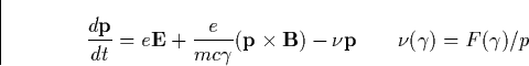
In the presence of a magnetic field the conditions for electron runaway are
different from those described for a pure static electric field. In order to
discuss the effects caused by magnetic field we will study the motion of
fast electrons in the air under the influence of both electric ![]() and magnetic field
and magnetic field ![]() . The equation of motion can be found from
the Boltzmann equation, Eq. (5.6), and is given by
. The equation of motion can be found from
the Boltzmann equation, Eq. (5.6), and is given by
 |
(17) |
 |
(18) |
 |
(19) |
![]()
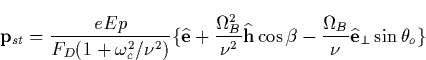
In the absence of magnetic field (B=0) Eq. (5.9) determines two
stationary points at E>Ec0. The first of these points is reached for pst<pmin given by Eq. (5.2). This is an unstable point. It
means that the electrons having p<pst are decelerated, while the
electrons with p>pst are accelerated and run away. The mentioned above
limit is correct for the momentum parallel to the electric field. If the
initial electron momentum possesses a component orthogonal to ![]() ,a separatrix appears which separates the runaway electrons from those losing
their energy [Gurevich et al., 1992; Roussel-Dupre et al.,
1994]. The same picture is correct if the constant magnetic field
,a separatrix appears which separates the runaway electrons from those losing
their energy [Gurevich et al., 1992; Roussel-Dupre et al.,
1994]. The same picture is correct if the constant magnetic field ![]() exists which is parallel to
exists which is parallel to ![]() . However, if a component of
. However, if a component of ![]() orthogonal to
orthogonal to ![]() appears, it can significantly change
the above picture. Let us consider a case when
appears, it can significantly change
the above picture. Let us consider a case when ![]()
![]() . We first introduce the dimensionless
. We first introduce the dimensionless
![]()
| |
(20) |
![]()
![\begin{figure}
\center
\includegraphics [1in,6.5in]
[6in,9in]{images/run_5.ps}\end{figure}](img396.gif) |
We find now the asymptotic form for ![]() at high values of
at high values of ![]() . In order to do it we take into account that at high
. In order to do it we take into account that at high ![]() the
value (v/c)2
the
value (v/c)2 ![]() 1, so the nonrelativistic dynamical friction force
can be applied. Therefore the function
1, so the nonrelativistic dynamical friction force
can be applied. Therefore the function ![]() is rewritten as
is rewritten as
 |
(21) |
The asymptote given by Eq. (5.11) is shown by a dashed trace in Fig.
5.5. The above discussion was focused on an instructive case when ![]()
![]() . However, Eq. (5.9) allows us to
obtain the critical electric field
. However, Eq. (5.9) allows us to
obtain the critical electric field ![]() as a function of the
magnetic field
as a function of the
magnetic field ![]() for an arbitrary angle
for an arbitrary angle ![]() between the
directions of the electric and magnetic field. This is shown in Fig. 5.5. In fact, for
between the
directions of the electric and magnetic field. This is shown in Fig. 5.5. In fact, for ![]() the critical electric field
practically does not depend on the value of the magnetic field, which
resembles the runaway as it occurs in the absence of the magnetic field and
is driven by E||. Note that the runaway electron moves at an angle
the critical electric field
practically does not depend on the value of the magnetic field, which
resembles the runaway as it occurs in the absence of the magnetic field and
is driven by E||. Note that the runaway electron moves at an angle ![]() to the direction of the electric field, where the angle
to the direction of the electric field, where the angle ![]() is obtained from Eq. (5.8). In fact, for
is obtained from Eq. (5.8). In fact, for ![]()
![]() , i.e.
, i.e. ![]() it acquires the following form
it acquires the following form
We study next the equation of the electron motion in order to obtain the
separatrix between the two regimes: those electrons which possess
trajectories that take them to higher energies, and the other electrons
which possess trajectories leading to zero energy. Using the dimensionless
variables ![]() and
and ![]() Eq. (5.7) is presented as
Eq. (5.7) is presented as
 |
(22) |
![]()
In this case the momentum is fading along the axes z, so essentially
electrons are moving in the x-y plane. At low magnetic field ![]() two kind of trajectories occur depending on the initial conditions. An
electron having low initial energy will lose its energy and eventually
stops, while an electron having high enough initial energy runs away along
an almost linear trajectory in the
two kind of trajectories occur depending on the initial conditions. An
electron having low initial energy will lose its energy and eventually
stops, while an electron having high enough initial energy runs away along
an almost linear trajectory in the ![]() plane,
and gains the energy. This regime resembles the runaway process as it
happened in the absence of a magnetic field. The picture changes when the
magnetic field increases so that
plane,
and gains the energy. This regime resembles the runaway process as it
happened in the absence of a magnetic field. The picture changes when the
magnetic field increases so that ![]() . In this case three
different types of trajectories occur depending on the initial conditions,
as it shown in Fig. 5.6 along with the corresponding temporal
evolution of the electron kinetic energy. In some cases an energetic
electron starts in the ux-uy plane and then rapidly losses its energy
and eventually stops (top two panels of Fig. 5.6). In other cases
the electron along a spiral trajectory while the electron kinetic energy
rapidly increases (at
. In this case three
different types of trajectories occur depending on the initial conditions,
as it shown in Fig. 5.6 along with the corresponding temporal
evolution of the electron kinetic energy. In some cases an energetic
electron starts in the ux-uy plane and then rapidly losses its energy
and eventually stops (top two panels of Fig. 5.6). In other cases
the electron along a spiral trajectory while the electron kinetic energy
rapidly increases (at ![]() ) and reaches then its steady state value
after making several oscillations (Middle two panels of Fig. 5.6).
) and reaches then its steady state value
after making several oscillations (Middle two panels of Fig. 5.6).
![\begin{figure}
\center
\includegraphics [width=5in,height=4.0in]{images/run_7.eps}\end{figure}](img422.gif) |
This regime is strongly different from what happened in the absence of a
magnetic field where the runaway electrons reach very high energies, while
in the ![]() field a steady state can be reached at a
much smaller electron energy. We describe also the third kind of
trajectories when the electron moves along the spiral trajectory losing its
energy and eventually stops (Bottom two panels of Fig. 5.6).
field a steady state can be reached at a
much smaller electron energy. We describe also the third kind of
trajectories when the electron moves along the spiral trajectory losing its
energy and eventually stops (Bottom two panels of Fig. 5.6).
This happens when the uy momentum component reaches such negative value
that the first and second terms in right part of the first of Eqs. (5.12) cancel each other (![]() ) leading to
the exponential temporal decay of the ux component. This is followed by
the temporal decay of the uy component as comes from the second of Eqs. (
5.12). However, when relativistic electrons gain and lose energy they
can generate Bremsstrahlung emission, and might produce secondary runaway
electrons.
) leading to
the exponential temporal decay of the ux component. This is followed by
the temporal decay of the uy component as comes from the second of Eqs. (
5.12). However, when relativistic electrons gain and lose energy they
can generate Bremsstrahlung emission, and might produce secondary runaway
electrons.
We proceed by defining the separatrix as a line in the ![]() and
and ![]() plane which
separates the initial electron velocities leading to the runaway regime from
those leading to the electron deceleration in a given electric and magnetic
field. This is shown in Fig. 5.7 calculated for the normalized
electric field
plane which
separates the initial electron velocities leading to the runaway regime from
those leading to the electron deceleration in a given electric and magnetic
field. This is shown in Fig. 5.7 calculated for the normalized
electric field ![]() , and for few different values of normalized
magnetic field (
, and for few different values of normalized
magnetic field (![]() = 6.0, 6.5, 7.0, and 7.5). For each of these cases
the runaway process occurs for
= 6.0, 6.5, 7.0, and 7.5). For each of these cases
the runaway process occurs for ![]() located
inside the domain bounded by the corresponding runaway separatrix. Note that
when the applied magnetic field increases, the region of runaway shrinks.
Finally,
located
inside the domain bounded by the corresponding runaway separatrix. Note that
when the applied magnetic field increases, the region of runaway shrinks.
Finally, ![]() reaches the maximum value
reaches the maximum value ![]() (
( ![]() ) when
the runaway ceases. In fact, at
) when
the runaway ceases. In fact, at ![]() the runaway ceases at
the runaway ceases at ![]() , which is in a considerable agreement with the critical value
, which is in a considerable agreement with the critical value ![]() (see Fig. 5.5), found above by using
some simplifications.
(see Fig. 5.5), found above by using
some simplifications.
![\begin{figure}
\center
\includegraphics [width=5in,height=4.0in]{images/run_8.eps}
\vspace{-.5em}
\center\end{figure}](img431.gif) |
Note that a primary runaway electron is able to produce a secondary electron
which also runs away, if the kinetic energy of the primary electron is at
least twice that required for runaway. This is the condition of the runaway
breakdown [Gurevich et al., 1994]. The separatrix of runaway
breakdown is obtained as it was done for the runaways, but using an
additional condition that the steady state kinetic energy of the runaway
electron is twice as large as its initial value. It is shown in Fig. 5.7b for the same values of electric and magnetic field as in Fig. 5.7a. Since the requirements for runaway breakdown are stronger than for
just runaway, the corresponding domain is smaller than that for the
runaways. In fact the runaway discharge developed at ![]() ceases if
ceases if
![]() .
.
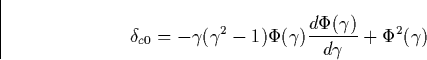
We consider now the runaway discharge stimulated by a seed high energy
electron. In the absence of the magnetic field the runaway discharge spreads
inside a cone stretched along the direction of the electric field [Gurevich et al., 1994]. Below we discuss how the magnetic field affects the
structure of the runaway discharge, and the dynamics of its spreading. We
concentrate mainly on the case when the electric and magnetic field are
parallel to each other. The motion of runaway electrons is studied in the
spherical coordinate frame, in which both E and B vectors are directed along
the x axis. The electron momentum evolves with an angle ![]() with the x
axis, while its projection on the plane z-y evolves with an angle
with the x
axis, while its projection on the plane z-y evolves with an angle ![]() with the y axis. In this frame Eqs. (5.12) can be represented as
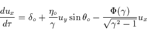
with the y axis. In this frame Eqs. (5.12) can be represented as
![\begin{displaymath}
\frac{du}{d\zeta }=\gamma [\delta _o\mu -\Phi (\gamma )] \end{displaymath}](img434.gif)
 |
(23) |
![\begin{displaymath}
\frac{du(\mu )}{d\mu }=\frac 1{\delta _o(1-\mu ^2)}[\delta _o\mu -\Phi
(\gamma (\mu ))] \end{displaymath}](img441.gif)
![]()
![\begin{figure}
\center
\includegraphics
*[1.0in,7.5in][5in,10in]{images/run_9.ps}\end{figure}](img444.gif) |
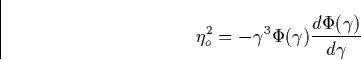
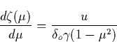
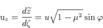
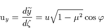
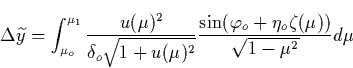
We consider next the diffusion of runaway electrons which occurs in the
plane perpendicular to ![]() , and caused by the fact that secondary
electrons appear at an arbitrarily angle. As a result of this diffusion the
runaway discharge caused by a single seed electron acquires a conical shape
as shown by Gurevich et al., [1994] in the absence of magnetic
field. The runaway electron possesses two velocity components in the (y, z)
plane
, and caused by the fact that secondary
electrons appear at an arbitrarily angle. As a result of this diffusion the
runaway discharge caused by a single seed electron acquires a conical shape
as shown by Gurevich et al., [1994] in the absence of magnetic
field. The runaway electron possesses two velocity components in the (y, z)
plane
![]()
![\begin{figure}
\center
\includegraphics
*[1in,7.0in][5in,10in]{images/run_10.ps}\end{figure}](img459.gif) |
In a general case when the angle between the vectors ![]() and
and ![]() is 0
is 0 ![]() 90, three different ranges of the angle
90, three different ranges of the angle ![]() were distinguished based on the physical properties of the
runaway process. They are illustrated by the runaway trajectories shown in
Figs. 5.10a, 5.10b, 5.10c obtained for different
were distinguished based on the physical properties of the
runaway process. They are illustrated by the runaway trajectories shown in
Figs. 5.10a, 5.10b, 5.10c obtained for different ![]() .
.
![\begin{figure}
\center
\includegraphics [width=3in,height=4in]{images/run_11.1.eps}
\includegraphics [width=2.5in,height=2in]{images/run_11.2.ps}\end{figure}](img461.gif) |
If the angle ![]() ranges between 80o and 90o the runaway
process differs significantly from that which occurs in the absence of the
magnetic field. First, it develops only if the ratio E/B is greater than a
certain threshold value, as was shown in Section 2. Second, contrary to the
runaway electrons in the absence of the magnetic field where the energy gain
is almost unlimited [ Roussel-Dupre et al., 1994], runaway
electrons at 80 o
ranges between 80o and 90o the runaway
process differs significantly from that which occurs in the absence of the
magnetic field. First, it develops only if the ratio E/B is greater than a
certain threshold value, as was shown in Section 2. Second, contrary to the
runaway electrons in the absence of the magnetic field where the energy gain
is almost unlimited [ Roussel-Dupre et al., 1994], runaway
electrons at 80 o ![]() 90o reach a steady state, at which
point they orbit across the magnetic field with a constant kinetic energy,
as it is shown in Fig. 5.10a obtained for
90o reach a steady state, at which
point they orbit across the magnetic field with a constant kinetic energy,
as it is shown in Fig. 5.10a obtained for ![]() = 85o.
= 85o.
In the range of 0o ![]() 60o the runaway process resembles
that which occurs in the absence of magnetic field, namely the electrons are
moving along the direction of the magnetic field driven by a E||
component of the electric field. This is illustrated by Fig. 5.10b,
obtained at
60o the runaway process resembles
that which occurs in the absence of magnetic field, namely the electrons are
moving along the direction of the magnetic field driven by a E||
component of the electric field. This is illustrated by Fig. 5.10b,
obtained at ![]() = 60o. The latter resembles a trajectory which is
almost a straight line in the (px,py,pz) space with a small effect of
magnetic field at low momentum. However, in this case the magnetic field
manifests itself by confining the runaway process, as discussed in Section 4.
= 60o. The latter resembles a trajectory which is
almost a straight line in the (px,py,pz) space with a small effect of
magnetic field at low momentum. However, in this case the magnetic field
manifests itself by confining the runaway process, as discussed in Section 4.
In the transient range 60o ![]() 80o the runaway electron
trajectories are twisted by the magnetic field when the electrons start the
acceleration and have relatively low energy. The electron then gains energy
along a straight trajectory, as shown by Fig. 5.10c obtained at
80o the runaway electron
trajectories are twisted by the magnetic field when the electrons start the
acceleration and have relatively low energy. The electron then gains energy
along a straight trajectory, as shown by Fig. 5.10c obtained at ![]() .
.
The effect caused by the angle between the electric and magnetic fields on
the runaway process is also illustrated by Fig. 5.11, which reveals
the kinetic energy of a runaway electron as a function of the angle ![]() . The kinetic energy was calculated for same initial conditions, and for
the time equal to that required to reach a steady state at
. The kinetic energy was calculated for same initial conditions, and for
the time equal to that required to reach a steady state at ![]() =90o. Note that
=90o. Note that ![]() has
a small, but finite value, in fact at
has
a small, but finite value, in fact at ![]() it is of the
order of 10-2.
it is of the
order of 10-2.
![\begin{figure}
\center
\includegraphics
*[1in,7.2in][6in,9.4in]{images/run_12.ps}\end{figure}](img466.gif) |
Figure 5.11 shows that at ![]() (i.e.
(i.e. ![]() ) the runaway is driven mostly by the
) the runaway is driven mostly by the ![]() component of
the electric field, and it is not strongly different from that which
occurred in the absence of a magnetic field; while at 0 < cos
component of
the electric field, and it is not strongly different from that which
occurred in the absence of a magnetic field; while at 0 < cos ![]() 0.16 (i.e. at 80o
0.16 (i.e. at 80o ![]() 90o) the effect of the magnetic field
becomes very important; and at 0.16
90o) the effect of the magnetic field
becomes very important; and at 0.16 ![]() 0.5 (i.e. at 60o
0.5 (i.e. at 60o ![]() 80o) a transient region between these two regimes exists.
80o) a transient region between these two regimes exists.
The runaway boundary for an arbitrarily angle ![]() could also be
investigated using the following approach. We consider an ensemble of N0
electrons moving in air in the presence of electric and magnetic fields. The
electrons which don't interact with each other, are uniformly distributed in
space, as well as in the energy range, which we consider for definiteness as
1
could also be
investigated using the following approach. We consider an ensemble of N0
electrons moving in air in the presence of electric and magnetic fields. The
electrons which don't interact with each other, are uniformly distributed in
space, as well as in the energy range, which we consider for definiteness as
1 ![]() 3.2. The trajectories of the electrons were studied using Eqs.
(5.12), and the trajectories which take electrons to higher energy
were then distinguished from those which lead to zero energy. Figure 5.12 reveals the fraction of electrons, N/N0, that runaway, as a
function of
3.2. The trajectories of the electrons were studied using Eqs.
(5.12), and the trajectories which take electrons to higher energy
were then distinguished from those which lead to zero energy. Figure 5.12 reveals the fraction of electrons, N/N0, that runaway, as a
function of ![]() . The calculation was made for the angle
. The calculation was made for the angle ![]() =
90o, and from left to right the value of
=
90o, and from left to right the value of ![]() changes from 0 to 10
with the step 1. In the absence of magnetic field, shown by the very left
trace, the separatrix resembles that obtained by Roussel-Dupre et al. [1994], while the increase of the magnetic field leads to the significant
reduction in the fraction of runaway electrons.
changes from 0 to 10
with the step 1. In the absence of magnetic field, shown by the very left
trace, the separatrix resembles that obtained by Roussel-Dupre et al. [1994], while the increase of the magnetic field leads to the significant
reduction in the fraction of runaway electrons.
![\begin{figure}
\center
\includegraphics [width=5in,height=3in]{images/run_13.eps}\end{figure}](img473.gif) |
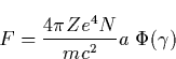
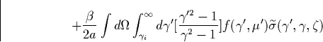
Finally, knowing the electron runaway boundary, one can find the characteristic ionization time in the discharge caused by the runaway electrons by using the fluid approximation, assuming that the electron distribution function is a delta-function, i.e. consider a monoenergetic flux of electrons. Note that of particular interested is the production rate of secondary runaway electrons, since their production leads to the development of the runaway breakdown.
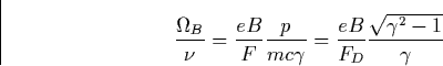
We state now the main features regarding the behavior of runaway electrons in the constant magnetic field.
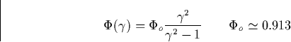
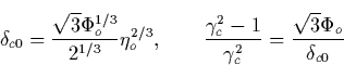
![]()
![]()
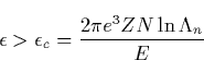
Since the critical field Ec0 is approximately an order of magnitude
less than the threshold of the conventional breakdown, it follows from the
last equation that in a case of perpendicular electric and magnetic fields
the runaway breakdown is hardly possible if ![]() .
.
In conclusion, the role played by the geomagnetic field in the runaway
process discussed above for heights less than 20 km is negligible.
Nevertheless the geomagnetic field plays a noticeable role at heights which
ranges from 20 to 30 km. In fact, it significantly changes the threshold
electric field E![]() for
for ![]() . At the height above 40 km
the effect of geomagnetic field dominates at large angles
. At the height above 40 km
the effect of geomagnetic field dominates at large angles ![]() and
the conditions of runaway breakdown becomes even more hindered.
and
the conditions of runaway breakdown becomes even more hindered.
Therefore at high altitudes, (z > 40 km) for angles ![]() between
between ![]() and
and ![]() close to
close to ![]() /2, the runaway breakdown is
hindered, while for
/2, the runaway breakdown is
hindered, while for ![]() between
between ![]() and
and ![]() , the runaway process can proceed freely. Thus taking into consideration
that the static electric field due to thunderclouds is directed almost
vertically one can expect a significant difference in the parameters of high
altitude discharges as they occur in the equatorial and midlatitudes.
, the runaway process can proceed freely. Thus taking into consideration
that the static electric field due to thunderclouds is directed almost
vertically one can expect a significant difference in the parameters of high
altitude discharges as they occur in the equatorial and midlatitudes.
Finally, we obtained the runaway separatrix which separates momentum space
into two regimes: those electrons which possess trajectories that take them
into higher energies, and other electrons which possess trajectories leading
to zero energy. Using this separatrix, the characteristic ionization time
required for the creation of a secondary runaway electron can be estimated.
![\begin{figure}
\center
\includegraphics [width=5in,height=4in]{images/run_4.eps}\end{figure}](img331.gif)
![\begin{figure}
\center
\includegraphics [width=5in,height=3in]{images/run_3.eps}\end{figure}](img354.gif)