First we start by computing the array factor based on the far field
approximation (see Appendix A). We take n and
and  and
compute the array factor at a height z=60 km. Figure 19 shows the
array factor for the discharge structure shown in Fig. 17 with
and
compute the array factor at a height z=60 km. Figure 19 shows the
array factor for the discharge structure shown in Fig. 17 with  .
.
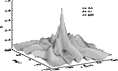
Figure 19: The array factor for  .
.
The length of the elementary current elements is about 100 m. The array
factor shows clear structure. A cross-section of the normalized array factor
are shown in Fig. 20 and Fig. 21 for  and
and  respectively.
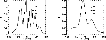
Figure 21: Cross-section of the array factor for 
Figure 20: Cross-section of the array factor for 
Similarly, the array factor at x=10 km, y=10 km, z=60 km is shown as a
function of the fractal dimension of the discharges for  and
and  in Fig. 22a for n
 and Fig. 22b
for n
and Fig. 22b
for n .
.
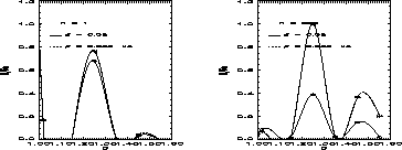
Figure 22: The array factor (a) For n and (b) for n
 . The graph
has been interpolated for the purpose of illustration.
. The graph
has been interpolated for the purpose of illustration.
The fractal dimension dependence of the array factor is very intriguing, but
is of clear significance for our lightning studies. What about the time
dependence of the radiations fields? Figure 23 shows the time
dependence of the radiation fields for 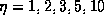 with n
 where each figure is carefully labeled.

Figure 23: The time dependence of the radiation fields for the fractal models.
See explanation in text.
Again the relevance of the  case is very striking. Each column of
graphs represent the time dependence for n
case is very striking. Each column of
graphs represent the time dependence for n respectively, where
the rows represent the case for
respectively, where
the rows represent the case for  . The amplitude of the
field has been multiplied by the factor displayed next to the graph.
. The amplitude of the
field has been multiplied by the factor displayed next to the graph.
We take the case for  and we study the dependence of the array
factor as a function of the current frequency as parametrized by n
and we study the dependence of the array
factor as a function of the current frequency as parametrized by n Figure 24 shows the frequency dependence of the array factor at
this location x=10 km, y=10 km, z=60 km. Initially the array factor
increases linearly with n
Figure 24 shows the frequency dependence of the array factor at
this location x=10 km, y=10 km, z=60 km. Initially the array factor
increases linearly with n as expected but then it starts to oscillate as
the spatial variation of the field pattern becomes relevant.
as expected but then it starts to oscillate as
the spatial variation of the field pattern becomes relevant.

Figure 24: The array factor as a function of  for
for 
In conclusion, the fractal nature of the discharges, being a simple random walk or a stochastic discharge model, leads naturally to an increase in the peak power density as compared with the dipole model. This increase is related to the increase in the antenna path length, or tortuosity, and on the branching process. It will be shown later that this gain in peak power density leads to a significant reductions in the discharge properties (e.g. charge, peak current) required to produce the observed sprite emissions. Furthermore, if the discharge has a high frequency component, as expected from an acceleration and deceleration process in each of the single steps, then the radiation pattern can show spatial structure. This spatial structure of the lightning induced radiation pattern will be related to the spatial structure of the red sprites in the next chapter.